Dissertation Example -A FRAMEWORK FOR MANAGEMENT OF DISTRIBUTED DATA PROCESSING AND EVENT SELECTION FOR THE ICECUBE NEUTRINO OBSERVATORY

A FRAMEWORK FOR MANAGEMENT OF DISTRIBUTED DATA PROCESSING
AND EVENT SELECTION FOR THE ICECUBE NEUTRINO OBSERVATORY
by
Juan Carlos Díaz Vélez
A thesis
submitted in partial fulfillment
of the requirements for the degree of
Master of Science in Computer Science
Boise State University
August 2013
c 2013
Juan Carlos D´ıaz V´elez
ALL RIGHTS RESERVED
BOISE STATE UNIVERSITY GRADUATE COLLEGE
DEFENSE COMMITTEE AND FINAL READING APPROVALS
of the thesis submitted by
Juan Carlos D´ıaz V´elez
Thesis Title: A Framework for management of distributed data processing and event selection for the IceCube Neutrino Observatory
Date of Final Oral Examination: 22 May 2013
The following individuals read and discussed the thesis submitted by student Juan Carlos D´ıaz V´elez, and they evaluated his presentation and response to questions during the final oral examination. They found that the student passed the final oral examination.
Amit Jain, Ph.D. Chair, Supervisory Committee
Jyh-haw Yeh, Ph.D. Member, Supervisory Committee
Alark Joshi, Ph.D. Member, Supervisory Committee
Daryl Macomb, Ph.D. Member, Supervisory Committee
The final reading approval of the thesis was granted by Amit Jain, Ph.D., Chair, Supervisory Committee. The thesis was approved for the Graduate College by John R. Pelton, Ph.D., Dean of the Graduate College.
ACKNOWLEDGMENTS
The author wishes to express gratitude to Dr. Amit Jain and the members of the committee as well the members of the IceCube Collaboration. The author also acknowledges the support from the following agencies: U.S. National Science Foundation-Office of Polar Programs, U.S. National Science Foundation-Physics Division, University of Wisconsin Alumni Research Foundation, the Grid Laboratory of Wisconsin (GLOW) grid infrastructure at the University of Wisconsin- Madison, the Open Science Grid (OSG) grid infrastructure; U.S. Department of Energy, and
National Energy Research Scientific Computing Center, the Louisiana Optical Net work Initiative (LONI) grid computing resources; National Science and Engineering Research Council of Canada; Swedish Research Council, Swedish Polar Research Secretariat, Swedish National Infrastructure for Computing (SNIC), and Knut and Alice Wallenberg Foundation, Sweden; German Ministry for Education and Research (BMBF), Deutsche Forschungsgemeinschaft (DFG), Research Department of Plasmas with Complex Interactions (Bochum), Germany; Fund for Scientific Research (FNRS-FWO), FWO Odysseus programme, Flanders Institute to encourage scientific
and technological research in industry (IWT), Belgian Federal Science Policy Office (Belspo); University of Oxford, United Kingdom; Marsden Fund, New Zealand; Japan Society for Promotion of Science (JSPS); the Swiss National Science Foundation (SNSF), Switzerland; This research has been enabled by the use of computing re sources provided by WestGrid and Compute/Calcul Canada.
AUTOBIOGRAPHICAL SKETCH
Juan Carlos was born and raised in Guadalajara, Jal. Mexico. He initially came to the U. S. as a professional classical ballet dancer and performed with several ballet companies including Eugene Ballet and Ballet Idaho. In 1996, Juan Carlos returned to school and graduated from Boise State University with a B. S. in Physics specializing
in Condensed Matter Theory under Dr. Charles Hanna where he was introduced to computation. Juan Carlos currently works for the IceCube Neutrino Observatory at the University of Wisconsin-Madison. In 2010, he traveled to the South Pole to work on the completion of the IceCube Detector.
ABSTRACT
IceCube is a one-gigaton neutrino detector designed to detect high-energy cosmic neutrinos. It is located at the geographic South Pole and was completed at the end of 2010. Simulation and data processing for IceCube requires a significant amount of computational power. We describe the design and functionality of IceProd, a management system based on Python, XMLRPC, and GridFTP. It is driven by a central database in order to coordinate and administer production of simulations and processing of data produced by the IceCube detector upon arrival in the northern hemisphere. IceProd runs as a separate layer on top of existing middleware and can take advantage of a variety of computing resources including grids and batch systems such as GLite, Condor, NorduGrid, PBS, and SGE. This is accomplished by a set of dedicated daemons that process job submission in a coordinated fashion through the
use of middleware plug-ins that serve to abstract the details of job submission and job management. IceProd fills a gap between the user and existing middleware by making job scripting easier and collaboratively sharing productions more efficiently.
We describe the implementation and performance of an extension to the IceProd framework that provides support for mapping workflow diagrams or DAGs consisting of interdependent tasks to an IceProd job that can span across multiple grid or cluster sites. We look at some use-cases where this new extension allows for optimal allocation of computing resources and addresses general aspects of this design, including security, data integrity, scalability, and throughput.
TABLE OF CONTENTS
ABSTRACT………………………………………..
LIST OF TABLES……………………………………
LIST OF FIGURES…………………………………..
LIST OF ABBREVIATIONS……………………………
1 Introduction………………………………………
1.1 IceCube . .. . . .. . . .. . . . .. . . .. . . . .. . . .. . . .. . . . .. . . .. . . .. . . .
1.1.1 Ice Cube Computing Resources .. . . .. . . .. . . . .. . . .. . . .. . . .
2 Ice Prod …………………………………………
2.1 Ice Prod. . .. . . .. . . .. . . . .. . . .. . . . .. . . .. . . .. . . . .. . . .. . . .. . . .
2.2 Design Elements of Ice Prod . . . .. . . . .. . . .. . . .. . . . .. . . .. . . .. . . .
2.2.1 Ice Prod Core Package . . .. . . . .. . . .. . . .. . . . .. . . .. . . .. . . .
2.2.2 Ice Prod Server. . . . .. . . .. . . . .. . . .. . . .. . . . .. . . .. . . .. . . .
2.2.3 Ice Prod Modules . . .. . . .. . . . .. . . .. . . .. . . . .. . . .. . . .. . . .
2.2.4 Client . .. . . .. . . . .. . . .. . . . .. . . .. . . .. . . . .. . . .. . . .. . . .
2.3 Database. .. . . .. . . .. . . . .. . . .. . . . .. . . .. . . .. . . . .. . . .. . . .. . . .
2.3.1 Database Structure .. . . .. . . . .. . . .. . . .. . . . .. . . .. . . .. . . .
2.4 Monitoring . . . .. . . .. . . . .. . . .. . . . .. . . .. . . .. . . . .. . . .. . . .. . . .
2.4.1 Web Interface . . . . .. . . .. . . . .. . . .. . . .. . . . .. . . .. . . .. . . .
2.4.2 Statistical Data.. . .. . . .. . . . .. . . .. . . .. . . . .. . . .. . . .. . . .
2.5 Security and Data Integrity . . . .. . . . .. . . .. . . .. . . . .. . . .. . . .. . . .
2.5.1 Authentication . . . .. . . .. . . . .. . . .. . . .. . . . .. . . .. . . .. . . .
2.5.2 Encryption . .. . . . .. . . .. . . . .. . . .. . . .. . . . .. . . .. . . .. . . .
2.5.3 Data Integrity. . . . .. . . .. . . . .. . . .. . . .. . . . .. . . .. . . .. . . .
2.6 Off-line Processing . .. . . . .. . . .. . . . .. . . .. . . .. . . . .. . . .. . . .. . . .
3 Directed A cyclic Graph Jobs………………………….
3.1 Condor DAG Man. . .. . . . .. . . .. . . . .. . . .. . . .. . . . .. . . .. . . .. . . .
3.2 Applications of DAGs:GPU Tasks . . .. . . .. . . .. . . . .. . . .. . . .. . . .
3.3 DAG sin Ice Prod . . .. . . . .. . . .. . . . .. . . .. . . .. . . . .. . . .. . . .. . . .
4 The Ice Prod DAG………………………………….
4.1 Design. . . .. . . .. . . .. . . . .. . . .. . . . .. . . .. . . .. . . . .. . . .. . . .. . . .
4.1.1 The Ice Prod DAG Class. .. . . . .. . . .. . . .. . . . .. . . .. . . .. . . .
4.1.2 The Task Q Class. . .. . . .. . . . .. . . .. . . .. . . . .. . . .. . . .. . . .
4.1.3 Local Database . . . .. . . .. . . . .. . . .. . . .. . . . .. . . .. . . .. . . .
4.2 Attribute Matching .. . . . .. . . .. . . . .. . . .. . . .. . . . .. . . .. . . .. . . .
4.3 Storing Intermediate Output . . .. . . . .. . . .. . . .. . . . .. . . .. . . .. . . .
4.3.1 Zones. . .. . . .. . . . .. . . .. . . . .. . . .. . . .. . . . .. . . .. . . .. . . .
5 Performance………………………………………
5.1 Experimental Setup .. . . . .. . . .. . . . .. . . .. . . .. . . . .. . . .. . . .. . . .
5.2 Performance . . .. . . .. . . . .. . . .. . . . .. . . .. . . .. . . . .. . . .. . . .. . . .
5.2.1 Task Queueing . . . .. . . .. . . . .. . . .. . . .. . . . .. . . .. . . .. . . .
5.2.2 Task Dependency Checks . . . . .. . . .. . . .. . . . .. . . .. . . .. . . .
5.2.3 Attribute Matching. . . . .. . . . .. . . .. . . .. . . . .. . . .. . . .. . . .
5.2.4 Load Balancing. . . .. . . .. . . . .. . . .. . . .. . . . .. . . .. . . .. . . .
6 Artifacts…………………………………………
6.1 Code. . . . .. . . .. . . .. . . . .. . . .. . . . .. . . .. . . .. . . . .. . . .. . . .. . . .
6.2 Documentation.. . . .. . . . .. . . .. . . . .. . . .. . . .. . . . .. . . .. . . .. . . .
7 Limitations of Ice Prod ………………………………
7.1 Fault Tolerance. . . . .. . . . .. . . .. . . . .. . . .. . . .. . . . .. . . .. . . .. . . .
7.2 Database Scalability.. . . . .. . . .. . . . .. . . .. . . .. . . . .. . . .. . . .. . . .
7.3 Scope of Ice Prod. . . .. . . . .. . . .. . . . .. . . .. . . .. . . . .. . . .. . . .. . . .
8 Conclusions ………………………………………
8.1 FutureWork. . .. . . .. . . . .. . . .. . . . .. . . .. . . .. . . . .. . . .. . . .. . . .
REFERENCES………………………………………
APython Package Dependencies…………………………
BJob Dependencies ………………………………….
CWritingan I3 Queue Plugina for New Batch System………..
DIce Prod Modules…………………………………..
D.1 PredefinedModules .. . . . .. . . .. . . . .. . . .. . . .. . . . .. . . .. . . .. . . .
D.1.1 DataTransfer . . . . .. . . .. . . . .. . . .. . . .. . . . .. . . .. . . .. . . .
E Experimental Sites Usedfor Testing Ice Prod DAG………….
E.0.2 WestGrid. . . .. . . . .. . . .. . . . .. . . .. . . .. . . . .. . . .. . . .. . . .
E.0.3 NERSC Dirac GPU Cluster . . .. . . .. . . .. . . . .. . . .. . . .. . . .
E.0.4 Center for High Throughput Computing(CHTC) . . .. . . .. . . .
E.0.5 University of Maryland’s Fear The Turtle Cluster. . . . .. . . .. . . .
F Additional Figures …………………………………
LIST OF TABLES
1.1 Data processing CPU. . . . .. . . .. . . . .. . . .. . . .. . . . .. . . .. . . .. . . .
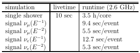
1.2 Runtime of various MC simulations.. . .. . . .. . . .. . . . .. . . .. . . .. . . .
4.1 Example zone definition for an Ice Prod instance .. . . . .. . . .. . . .. . . .
5.1 Sites participating in experimental Ice Prod DAG tests . .. . . .. . . .. . . .
5.2 Runtimes for task-queueing functions. . . . .. . . .. . . . .. . . .. . . .. . . .
5.3 Task run times .. . . .. . . . .. . . .. . . . .. . . .. . . .. . . . .. . . .. . . .. . . .
E.1 CHTC Resources . . .. . . . .. . . .. . . . .. . . .. . . .. . . . .. . . .. . . .. . . .
E.2 UMD Compute Cluster . . .. . . .. . . . .. . . .. . . .. . . . .. . . .. . . .. . . .
LIST OF FIGURES
1.1 The Ice Cubedetector. . . . .. . . .. . . . .. . . .. . . .. . . . .. . . .. . . .. . . .
2.1 JEP state diagram. .. . . . .. . . .. . . . .. . . .. . . .. . . . .. . . .. . . .. . . .
2.2 Network diagram of Ice Prod system. . .. . . .. . . .. . . . .. . . .. . . .. . . .
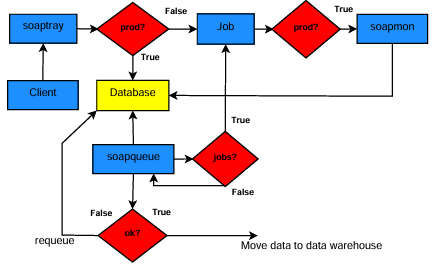
2.3 State diagram of queueing algorithm. .. . . .. . . .. . . . .. . . .. . . .. . . .
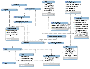
2.4 Diagram of database. . . . . .. . . .. . . . .. . . .. . . .. . . . .. . . .. . . .. . . .
3.1 Asimple DAG .. . . .. . . . .. . . .. . . . .. . . .. . . .. . . . .. . . .. . . .. . . .
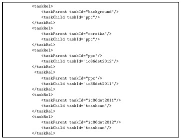
3.2 XML representation of a Dag.. .. . . . .. . . .. . . .. . . . .. . . .. . . .. . . .
3.3 A more complicated DAG .. . . .. . . . .. . . .. . . .. . . . .. . . .. . . .. . . .
4.1 Ice Prod DAG implementation . .. . . . .. . . .. . . .. . . . .. . . .. . . .. . . .
4.2 Task Q factory. .. . . .. . . . .. . . .. . . . .. . . .. . . .. . . . .. . . .. . . .. . . .
4.3 JEP state diagram for a task . . .. . . . .. . . .. . . .. . . . .. . . .. . . .. . . .
4.4 Task requirement expressions . . .. . . . .. . . .. . . .. . . . .. . . .. . . .. . . .
4.5 Distribution offile transfer speeds . . . .. . . .. . . .. . . . .. . . .. . . .. . . .
4.6 Distribution offile transfer speed over a long interval . .. . . .. . . .. . . .
4.7 Evolution of average transfer speed . . .. . . .. . . .. . . . .. . . .. . . .. . . .
4.8 SQL query with zone prioritization . . .. . . .. . . .. . . . .. . . .. . . .. . . .
5.1 DA Gused for benchmark in . . . .. . . . .. . . .. . . .. . . . .. . . .. . . .. . . .
5.2 Worst case scenario for dependency check algorithm in a DAG. . .. . . .
5.3 Examples of best cases scenario for dependency check algorithm in a DAG 48
5.4 Range of complexity for task dependency checks .. . . . .. . . .. . . .. . . .
5.5 Task completion by site . . .. . . .. . . . .. . . .. . . .. . . . .. . . .. . . .. . . .
5.6 Task completion by site(CPU tasks) . .. . . .. . . .. . . . .. . . .. . . .. . . .
5.7 Task completion by site(GPU tasks). .. . . .. . . .. . . . .. . . .. . . .. . . .
5.8 Ratio of CPU/GPU tasks for Dataset 9544 .. . . .. . . . .. . . .. . . .. . . .
C.1 I3 Queue implementation. . .. . . .. . . . .. . . .. . . .. . . . .. . . .. . . .. . . .
D.1 IP Module implementation .. . . .. . . . .. . . .. . . .. . . . .. . . .. . . .. . . .
F.1 The xice prod client. .. . . . .. . . .. . . . .. . . .. . . .. . . . .. . . .. . . .. . . .
F.2 Ice Prod Web Interface . . . .. . . .. . . . .. . . .. . . .. . . . .. . . .. . . .. . . .
LIST OF ABBREVIATIONS
DAG–Directed Acyclic Graph
DOM–Digital Optical Module
EGI– European Grid Initiative
GPU– Graphics Processing Unit
JEP– Job Execution Pilot
LDAP– Lightweight Directory Access Protocol
PBS– Portable Batch System
RPC–Remote Procedure Call
SGE– Sun Grid Engine
XML–Extensive Markup Language
XMLRPC–HTTP based RPC protocol with XML serialization
CHAPTER 1
INTRODUCTION
Large experimental collaborations often need to produce large volumes of computationally intensive Monte Carlo simulations and process vast amounts of data. These tasks are often easily farmed out to large computing clusters, or grids but for such large datasets it is important to be able to document software versions and parameters
including pseudo-random number generator seeds used for each dataset produced. Individual members of such collaborations might have access to modest computational resources that need to be coordinated for production. Such computational resources could also potentially be pooled in order to provide a single, more powerful, and
more productive system that can be used by the entire collaboration. Ice Prod is a scripting framework package meant to address all of these concerns. It consists of queuing daemons that communicate via a central database in order to coordinate production of large datasets by integrating small clusters and grids [3]. The core objective of this Master’s thesis is to extend the functionality of Ice Prod to include a workflow management DAG tool that can span multiple computing clusters and/or grids. Such DAGs will allow for optimal use of computing resources.
1.1 Ice Cube
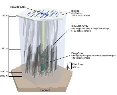
The IceCube detector shown in Figure 1.1 consists of 5160 optical sensors buried between 1450 and 2450 meters below the surface of the South Polar ice sheet and is designed to detect neutrinos from astrophysical sources [1, 2]. However, it is also sensitive to downward-going muons produced in cosmic ray air showers with energies
in excess of several TeV1. IceCube records ∼1010 cosmic-ray events per year. These cosmic-ray-induced muons represent a background for most IceCube analyses as they outnumber neutrino-induced events by about 500 000:1 and must be filtered prior to transfer to the northern hemisphere due to satellite bandwidth limitations [4]. In
order to develop reconstructions and analyses, and in order to understand systematic uncertainties, physicists require a comparable amount of statistics from Monte Carlo simulations. This requires hundreds of years of CPU processing time.
1.1.1 IceCube Computing Resources
The IceCube collaboration is comprised of 38 research institutions from Europe, North America, Japan, and New Zealand. The collaboration has access to 25 different clusters and grids in Europe, Japan, Canada, and the U.S. These range from small computer farms of 30 nodes to large grids such as the European Grid Infrastructure (EGI), European Enabling Grids for E-sciencE (EGEE), Louisiana Optical Network Initiative (LONI), Grid Laboratory of Wisconsin (GLOW), SweGrid, Canada’s West Grid, and the Open Science Grid (OSG) that may each have thousands of compute nodes. The total number of nodes available to IceCube member institutions is uncertain since much of our use is opportunistic and depends on the usage by other
11 TeV = 1012 electron-volts (unit of energy)
projects and experiments. In total, IceCube simulation has run on more than 11,000 distinct nodes and a number of CPU cores between 11,000 and 44,000. On average, IceCube simulation production has run concurrently on ∼4,000 cores at a given time and it is anticipated to run on ∼5,000 cores simultaneously during upcoming productions.
Table 1.1: Data processing demands. Data is filtered on 400 cores at the South Pole using loose cuts to reduce volume by a factor of 10 before satellite transfer to the northern hemisphere (Level1). Once in the North, more computationally intensive event reconstructions are performed in order to further reduce background contamination (Level2). Further event selections are made for each analysis channel (Level3).
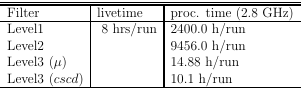
Table 1.2: Runtime of various MC simulations of background cosmic-ray shower events and neutrino (ν) signal with different energy spectra for different flavors of neutrinos.
CHAPTER 2
ICEPROD
2.1 IceProd
The IceProd framework is a software package developed for the IceCube collaboration in order to address the needs for managing productions across distributed systems and in order to pool resources scattered throughout the collaboration [3]. It fills a gap between the powerful middleware and batch system tools currently available and the
user or production manager. It makes job scripting easier and collaboratively sharing productions more efficient. It includes a collection of interfaces to an expanding number of middleware and batch systems that makes it unnecessary to re-write scripting code when migrating from one system to another. This Python-based distributed system consists of a central database and a set of daemons that are responsible for various roles on submission and management of grid jobs as well as data handling. IceProd makes use of existing grid technology and network protocols in order to coordinate and administer production of simulations and processing of data. The details of job submission and management in different grid environments is abstracted through the use of plug-ins. Security and data integrity are concerns in any software architecture that depends heavily on communication through the Internet. IceProd includes features aimed at minimizing security and data corruption risks.
IceProd provides a graphical user interface (GUI) for configuring simulations and submitting jobs through a production server. It provides a method for recording all the software versions, physics parameters, system settings, and other steering parameters in a central production database. IceProd also includes an object-oriented web page written in PHP for visualization and live monitoring of datasets. The package includes a set of libraries, executables, and daemons that communicate with the central database and coordinate to share responsibility for the completion of tasks. Because of this, IceProd can thus be used to integrate an arbitrary number of sites, including clusters and grids at the user level. It is not, however, a replacement for Globus, GLite, or any other middleware. Instead, it runs on top of these as a separate layer with additional functionality.
Many of the existing middleware tools including Condor-C, Globus, and CREAM make it possible to pool any number of computing clusters into a larger pool. Such arrangements typically require some amount of work by system administrators and may not be necessary for general purpose applications. Unlike most of these applications, IceProd runs at the user level and requires no administrator privileges. This makes it easy for individual users to build large production systems by pooling small computational resources together.
The primary design goal of IceProd was to manage production of IceCube detector simulation data and related filtering and reconstruction analyses but its scope is not limited to IceCube. Its is design general enough to be used for other applications. As of this writing, the Hight Altitude Water Cherenkov (HAWC) observatory has begun
using IceProd for off-line data processing [5]. Development of IceProd is an ongoing effort. One important current area of development is the implementation of workflow management capabilities like Condor’s
DAGManinorder to optimize the use of specialized hardware and network topologies by running different job sub-tasks on different nodes. The are two approaches to DAGs in the IceProd frame work. The first is a plug-in-based approach that relies on the existing workflow functionality of the batch system and the second, which is the product of this Master’s thesis is native IceProd implementation that allows a single job’s tasks to span multiple grids or clusters.
2.2 Design Elements of IceProd
The IceProd software package can be logically divided into the following components or software libraries illustrated in Figure 2.2:
• iceprod-core- a set of modules and libraries of common use throughout IceProd.
• iceprod-server- a collection of deamons and libraries to manage and schedule job submission and monitoring.
• iceprod-modules- a collection of predefined IceProdModule classes that provide an interface between IceProd and an arbitrary task to be performed on a compute node as will be defined in Section 2.2.3.
• iceprod-client- a client (both graphical and text) that can download, edit, and submit dataset steering files to be processed.
• Adatabase that stores configured parameters, libraries (including version information), job information, and performance statistics.
• Aweb application for monitoring and controlling dataset processing. The following sections will describe these components in further detail.
2.2.1 IceProd Core Package
The iceprod-core package contains modules and libraries common to all other IceProd packages. These include classes and methods for writing and parsing XML, trans porting data, and this is also where the basic classes that define a job execution on a host are themselves defined. Also included in this package is an interpreter for a simple scripting language that provides some flexibility to XML steering files.
The JEP
One of the complications of operating on heterogeneous systems is the diversity of architectures, operating systems, and compilers. For this reason, Condor’s NMI Metronome build and test system [6] is used for building the IceCube software for a variety of platforms. IceProd sends a Job Execution Pilot (JEP), a Python script that determines what platform it is running on, and after contacting the monitoring server determines which software package to download and execute. During runtime, this executable will perform status updates through the monitoring server via XMLRPC, a remote procedure call protocol that works over the Internet [7]. This information is updated on the database and is displayed on the monitoring web page. Upon completion, the JEP will clean up its workspace, but if configured to do so will cache a copy of the software used and make it available for future runs. When caching is
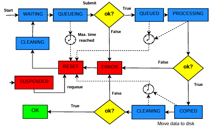
enabled, an MD5Sum check is performed on the cached software and compared to what is stored on the server in order to avoid using corrupted or outdated software. Jobs can fail under many circumstances. These can include submission failures due to transient system problems and execution failures due to problems with the execution host. At a higher level, errors specific to IceProd include communication problems with the monitoring daemon or the data repository. In order to account for possible transient errors, the design of IceProd includes a set of states through which a job will transition in order to guarantee a successful completion of a well-configured job. The state diagram for an IceProd job is depicted in Figure 2.1.
XML Job Description
In the context of this document, a dataset is defined to be a collection of jobs that share a basic set of scripts and software but whose input parameters depend on the enumerated index of the job. A configuration or steering file describes the tasks to be executed for an entire dataset. IceProd steering files are XML documents with a defined schema. This document includes information about the specific software versions used for each of the sections known as trays (a term borrowed from IceTray, the C++ software framework used by the IceCube collaboration [8]), parameters passed to each of the configurable modules, and input files needed for the job. In addition, there is a section for user-defined parameters and expressions to facilitate programming within the XML structure. This is discussed further in Section 2.2.1.
IceProd Expressions
A limited programming language was developed in order to allow more scripting flexibility that depends on runtime parameters such as job index, dataset ID, etc. This allows for a single XML job description to be applied to an entire dataset following a SPMD(Single Process, Multiple Data) operation mode. Examples of valid expressions include the following:
1. $args() a command line argument passed to the job (such as job ID, or dataset ID).
2. $steering() a user-defined variable.
3. $system() a system-specific parameter defined by the server.
4. $eval() a mathematical expression (Python).
5. $sprintf(,) string formatting.
6. $choice() random choice of element from list.
7. $attr() system-dependent attributes to be matched against IceProdDAG jobs (discussed in Chapter 4).
The evaluation of such expressions is recursive and allows for a fair amount of complexity. There are, however, limitations in place in order to prevent abuse of this feature. An example of this is that $eval() statements prohibit such things as loops and import statements that would allow the user to write an entire Python program
within an expression. There is also a limit on the number of recursions in order to prevent closed loops in recursive statements.
2.2.2 IceProd Server
The IceProd server is comprised of the four daemons mentioned in the list below (items 1-4) and their respective libraries. There are two basic modes of operation: the first is a non-production mode in which jobs are simply sent to the queue of a particular system, and the second stores all of the parameters in the database and also tracks the progress of each job. The soapqueue daemon running at each of the participating sites periodically queries the database to check if any tasks have been assigned to it. It then downloads the steering configuration and submits a given number of jobs. The size of the queue at each site is configured individually based on the size of the cluster and local queuing policies.
1. soaptray- a server that receives client requests for scheduling jobs and steering information.
2. soapqueue- a daemon that queries the database for tasks to be submitted to a particular cluster or grid.
3. soapmon- a monitoring server that receives updates from jobs during execution and performs status updates to the database.
4. soapdh- a data handler/garbage collection daemon that takes care of cleaning up and performing any post-processing tasks.
Figure 2.2 is a graphical representation that describes the interrelation of these daemons.
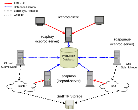
municate with iceprod-server modules via XMLRPC. Database calls are restricted to iceprod-server modules. Queueing daemons called soapqueue are installed at each site and periodically query the database for pending job requests. The soapman server receives monitoring update from the jobs.
Plug-ins
In order to abstract the process of job submission for the various types of systems, IceProd defines a base class I3Grid that provides an interface for queuing jobs. Plug-in sub-classes then implement the required functionality of each system and include
functions for queuing jobs, removing jobs, and status checks. Plug-ins also support the inclusion of job attributes such as priority, maximum allowed wall time, and requirements such as disk, memory, etc. IceProd has a growing library of plug-ins that are included with the software including Condor, PBS, SGE, Globus, GLite, Edg,
CREAM, SweGrid, and other batch systems. In addition, one can easily implement user-defined plug-ins for any new type of system that is not included in this list.
2.2.3 IceProd Modules
IceProd modules, like plug-ins, implement an interface defined by a base class IP Module. These modules represent the atomic tasks to be performed as part of the job. They have a standard interface that allows for an arbitrary set of parameters to be configured in the XML document and passed from the IceProd framework. In turn, the module returns a set of statistics in the form of a string-float dictionary back to the framework so that it can be automatically recorded in the database and displayed on the monitoring web page. By default, the base class will report the
module’s CPU usage but the user can define any set of values to be reported such as number of events that pass a given processing filter, etc. IceProd also includes a library of predefined modules for performing common tasks such as file transfers through GridFTP, tarball manipulation, etc.
External IceProd Modules
Included in the library of predefined modules is a special module i3, which has two parameters, class and URL. The first is a string that defines the name of an external IceProd module and the second specifies a Universal Resource Locator (URL) for a (preferably version-controlled) repository where the external module code can be
2.2.4 Client
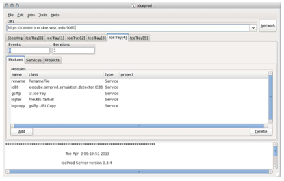
The IceProd-Client contains two applications for interacting with the server and submitting datasets. One is a pyGtk-based GUI (see Figure F.1) and the other is a text-based application that can run as a command-line executable or as an interactive shell. Both of these applications allow the user to download, edit, submit, and control datasets running on the IceProd-controlled grid. The graphical interface includes drag and drop features for moving modules around and provides the user with a list of valid parameter for know modules. Information about parameters for external modules is not included since these are not known a priori. The interactive shell also allows the user to perform grid management tasks such as starting and stopping a remote server, adding and removing participation of specific sites in the processing of a dataset, as well as job-specific actions such as suspend and reset.
2.3 Database
At the time of this writing, the current implementation of IceProd works exclusively with a MySQL database but all database calls are handled by a database module which abstracts queries and could be easily replaced by a different relational database. This section describes the relational structure of the IceProd database.
2.3.1 Database Structure
A dataset in IceProd represents a job description and a collection of jobs associated with. Each dataset describes a common set of modules and parameters but operate on separate data (single instruction, multiple data). At the top level of the database structure is the dataset table. The primary key database id is the unique identifier for each dataset though it is possible to assign nemonic string alias. Figure 2.4 is a simplified graphical representation of the relational structure of the database. The IceProd database is logically divided into two classes that could in principle be entirely different databases. The first describes a steering file or dataset configuration (items 1- 8 in the list below) and the second is a job-monitoring database (items 9- 12). The most important tables are described below.
1. dataset:
unique identifier as well as attributes to describe and categorize the dataset including a textual description.
2. meta project:
describes a software environment including libraries and executables.
3. module:
describes an IPModule class.
4. module pivot:
relates a module to a given dataset and specifies the order in which this module is called.
5. tray:
describes a grouping of modules that will execute given the same software environment or meta project
6. cparameter:
describes the name, type, and value of parameter associated with a module.
7. carray element:
describes an array element value in the case the parameter is of type vector or a name-value pair if the parameter is of type dict.
8. steering parameter:
describes general global variables that can be referenced from any module.
9. job:
describes each job in the queue related to a dataset. Columns include state, error msg, previous status, and last update.
10. task def:
describes a taks definition an related trays.
11. task rel:
describes the relationship of task definitions or task def s
12. task:
keeps track of the state of a task in a similar way that job does.
2.4 Monitoring
The status updates and statistics reported by the JEP via XMLRPC and stored in the database provide useful information for monitoring not only the progress of datasets but also for detecting errors. The monitoring daemon soapmon is an HTTP daemon that listens to XMLRPC requests from the running processes (instances of JEP). The
updates include status changes and information about the execution host as well as job statistics. This is a multi-threaded server that can run as a stand-alone daemon or as a cgi-bin script within a more robust Web server. The data collected from each job can be analyzed and patterns can be detected with the aid of visualization tools as described in the following section.
2.4.1 Web Interface
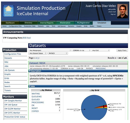
The current web interface for IceProd was designed by a collaborator, Ian Rae. It works independently from the IceProd framework but utilizes the same database. It is written in PHP and makes use of the CodeIgniter object-oriented framework [9]. The IceCube simulation and data processing web monitoring tools provide different views that include, from top level downwards,
• general view: displays all datasets filtered by status, type, grid, etc.
• grid view: displays everything that is running a particular site,
• dataset view: displays all jobs and statistics for a given dataset including every site that it is running on, and
• job view: displays each individual job including status, job statistics, execution host, and possible errors.
There are some additional views that are applicable only to the processing of real detector data:
• calendar view: displays a calendar with a color-coding indicating the status of job associated with a particular data-taking day.
• day view: displays the status of detector runs for a given calendar day.
• run view: displays the status of jobs associated with a particular detector run.
The web interface also uses XMLRPC in order to send commands to the soaptray daemon and provides authenticated users the ability to control jobs and datasets. Other features include graphs displaying completion rates, errors, and number of jobs in various states.
2.4.2 Statistical Data
One aspect of IceProd that is not found in most grid middleware is the built-in collection of user-defined statistical data. Each IceProd module is passed a <string,float> map object to which it can add entries or increment a given value. IceProd collects this data on the central database and reports it on the monitoring page individually
for each job and collectively for the whole dataset as a sum, average, and standard deviation. The typical type of information collected on IceCube jobs includes CPU usage, number of events passing a particular filter, number of calls to a particular module, etc.
2.5 Security and Data Integrity
Whenever dealing with network applications one must always be concerned with security and data integrity in order to avoid compromising privacy and the validity of scientific results. Some effort has been made to minimize security risks in the design and implementation of IceProd. This section will summarize the most significant of these. Figure 2.2 indicates the various types of network communication between the client, server, and worker node.
2.5.1 Authentication
IceProd integrates with an existing LDAP server for authentication. If one is not available, authentication can be done with database accounts though the former is preferred. Whenever LDAP is available, direct database authentication should be disabled. LDAP authentication allows the IceProd administrator to restrict usage to individual users that are responsible for job submissions and are accountable to improper use. This also keeps users from being able to directly query the database via a MySQL client.
2.5.2 Encryption
Both soaptray and soapmon can be configured to use SSL certificates in order to encrypt all data communication between client and server. The encryption is done by the HTTPS server with either a self-signed certificate or preferably with a certificate signed by a trusted CA. This is recommended for client-soaptray communication but is generally not considered necessary for monitoring information sent to soapmon by the JEP as this just creates a higher CPU load on the system.
2.5.3 Data Integrity
In order to guarantee data integrity, an MD5sum or digest is generated for each file that is transmitted. This information is stored in the database and is checked against the file after transfer. Data transfers support several protocols but preference is to primarily rely on GridFTP, which makes use of GSI authentication [10, 11]. When dealing with databases one also needs to be concerned about allowing direct access to the database and passing login credentials to jobs running on remote sites. For this reason, all monitoring calls are done via XMLRPC and the only direct queries are performed by the server, which typically operates behind a firewall on a trusted system. The current web design does make direct queries to the database but a dedicated read-only account is used for this purpose. An additional security measure is the use of a temporary random-generated string that is assigned to each job at the time of submission. This passkey is used for authenticating communication between the job and the monitoring server and is only valid during the duration of the job. If the job is reset, this passkey will be changed before a new job is submitted. This prevents stale jobs that might be left running from making monitoring updates after the job has been reassigned.
2.6 Off-line Processing
This section describes the functionality of IceProd that is specific to detector data processing. For Monte Carlo productions, the user typically defines the output to be generated including the number of files. This makes it easy to determine the size of a dataset a priori such that the job table is generated at submission time. Unlike Monte Carlo production, real detector data is typically associated with particular times and dates and the total size of the dataset is typically not know from the start. In IceCube, a dataset is divided in to experiment runs that span over ∼ 8 hours (see Table 1.1 on Page 3). Each run contains an variable number of sub-runs with files of roughly equal size.
A processing steering configuration generates an empty dataset with zero jobs. A separate script is then run over the data in order to map a file (or files) to a particular job as an input. Additional information is also recorded such as date, run number, and sub-run number mostly for display purposes on the monitoring web page but this information is not required for functionality of IceProd. Once this mapping has been generated, there is a processing-specific base class derived from Ice Prod Module that automatically gets a list of input files from the soapmon server. This list of files includes information such as URL, file size, MD5Sum, and type of file. The module then downloads the appropriate files and performs a checksum to make sure there was no data corruption during transmission. All output files are subsequently recorded on the database with similar information. The additional information about the run provides a calendar view on the monitoring page.
CHAPTER 3
DIRECTED ACYCLIC GRAPH JOBS
Directed acyclic graphs or DAGs allow you to define a job composed of multiple tasks that are to be run on separate compute nodes and may have inter dependencies. DAGs make it possible to map a large workflow problem into a set of jobs that may have different hardware requirements and to parallelize portions of the workflow. Examples of DAGs are graphically represented in Figures 3.1 and 3.3.
3.1 Condor DAGMan
DAGMan is a workflow manager developed by the HTCondor group at University of Wisconsin-Madison and included in with the HTCondorTM batch system [12]. Condor DAGMan describes job dependencies as directed acyclic graphs. Each vertex in the graph represents a single instance of a batch job to be executed while edges correspond the execution order of the jobs or vertices. A DAGMan submit script describes the relationships of vertices and associates a Condor submit script for each vertex or task.
3.2 Applications of DAGs: GPU Tasks
The instrumented volume of ice at the South Pole is an ancient glacier that has formed over several thousands of years. As a result, it has a layered structure of scattering and absorption coefficients that is complicated to model. Recent developments in IceCube’s simulation include a much faster approach for direct propagation of photons in the optically complex Antarctic ice [13] by use of GPUs. This new simulation module runs much faster than a CPU-based implementation and more accurately than using parametrization tables [14], but the rest of the simulation requires standard CPUs. As of this writing, IceCube has access to ∼ 20k CPU cores distributed throughout the world but has only a small number of nodes equipped with GPU cards. The entire simulation cannot be run on the GPU nodes since it is CPU bound and would be too slow in addition to wasting valuable GPU resources. In order to
solve this problem, the DAG feature in IceProd is used along with the modular design of the IceCube simulation chain in order to assign CPU tasks to general purpose grid nodes while running the photon propagation on GPU-enabled machines as depicted in Figure 3.1.
3.3 DAGs in IceProd
The original support for DAGs in IceProd was through Condor’s DAGMan and was implemented by Ian Rae, a colleague from University of Wisconsin. The Condor plug in for IceProd provides an interface for breaking up a job into multiple interdependent tasks. In addition to changes required in the plug-in, it was necessary to add a way to
describe such a graph in the IceProd dataset XML steering file. This is accomplished by associating a given module sequence or tray to a task and declaring a parent/child association for each interdependent set of tasks as shown in Figures 3.1 and 3.2. Similar plug-ins have also been developed for PBS and Sun Grid Engine plug-ins. One limitation of this type of DAG is that it is restricted to run on a specific cluster and does not allow you to have tasks that are distributed across multiple sites.
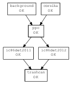
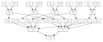
Figure 3.1: A simple DAG in IceProd. This DAG corresponds to a typical IceCube simulation. The two root nodes require standard computing hardware and produce different types of signal. Their output is then combined and processed on specialized hardware. The output is then used as input for two different detector simulations.
CHAPTER 4
THE ICEPROD DAG
The primary objective for this thesis has been to implement a DAG that is driven by IceProd and is independent from any batch system. This chapter describes the design and implementation of a workflow management system similar to Condor’s DAGMan that is primarily based on the plug-in feature of IceProd. There has been some work recently to incorporate work flow management DAGs into grid system. For example, Cao et al. have developed a sophisticated workflow manager that relies on performance modeling and predictions in order to schedule tasks [15]. By contrast, IceProd relies on a consumer-based approach to scheduling where local resources consume tasks on demand. This approach naturally lends itself to efficient utilization of computing resources.
4.1 Design
The IceProdDAG consists of a pair of plug-ins that take the roles of a master queue and a slave queue, respectively. The master queue interacts solely with the database rather than acting as an interface to a batch system while the slave task queue manages task submission via existing plug-in interfaces. Both of these classes are implemented in a plug-in module simply called dag.py. In order to implement this design, it was also necessary to write some new methods for the database module and to move several database calls such that they are called from within the plugin. These calls are now normally handled by the plug-in iGrid base class but are overloaded by the dag plug-in.
The current database design already includes a hierarchical structure for representing DAGs and this can be used for checking task dependencies. A major advantage of this approach is that it allows a single DAG to span multiple sites and thereby make optimal use of resources. An example application would allow to combine one site with vast amounts of CPU power but no GPUs available and another site better equipped with GPUs.
4.1.1 The IceProdDAG Class
The primary role of the IceProdDAG class is to schedule tasks and handle their respective inter-job dependencies. This class interacts with the database in order to direct the execution order of jobs on other grids. The IceProdDAG class assumes the existence of a list of sub-grids in its configuration. These are manually configured by the administrator, though in principle it is possible to dynamically extend a dataset to include other sub-grids via the database. The algorithm that determines inclusion or exclusion of a sub-grid in the execution of a task for a given dataset is described in Section 4.2.
The IceProdDAG plug-in queues jobs from the database just as any other batch system plug-in would but rather than writing submit scripts and submitting jobs to a cluster or grid, it updates the status of the child tasks associated with each job and leaves the actual job submission to the respective sub-grids. The pseudo-code in Figure 4.1 shows the main logic used for determining the execution order of tasks.
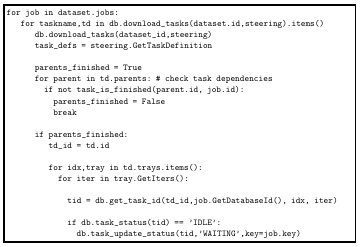
The initial state of all tasks is set to IDLE, which is equivalent to a hold state. When scheduling a new job, the IceProdDAG then traverses the dependency tree, starting with all tasks a level 0 until it finds a task that is ready to be released by meeting one of the following conditions:
1. The task has no parents (a level 0 task).
2. All the task parents have completed and are now in a state of OK.
If a task meets these requirements, its status is set to WAITING and any sub-grids that meet the task requirements is free to grab this task and submit it to its own scheduler. As with other plugins, the IceProdDAG will only keep track of a maximum sized set of “queued” jobs determined by the iceprod.cfg configuration.
4.1.2 The TaskQ Class
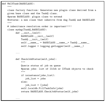
The TaskQ class is an abstract base class from which other plug-in classes can extend their own functionality by means of inheritance. This class treats the task as a single job rather than a component of one. TaskQ overloads many of the database method calls and handles treatment of a node in a DAG or task in the same way that the iGrid class and the derived plug-ins handle jobs. The implementation of batch system-specific plugins takes advantage of Python’s support for multiple inheritance [16]. In order to implement an IceProd-based dag on a system X, one can define a class Xdag that derives from both dag.TaskQ and X. The dag.TaskQ class provides the interaction to the database while class X provides the interface to the batch system. Inheritance order is important in order to properly resolve class methods. The dagmodule includes a TaskQ factory function (Figure 3.2) that can automatically define a new TaskQ-derived class for any existing plug-in. The IceProd administrator simply needs to specify a plug-in of type BASECLASS::TaskQ. The plug-in factory understands that it needs to generate an instance that is derived from BASECLASS and TaskQ with the proper methods overloaded when inheritance order needs to be overridden.
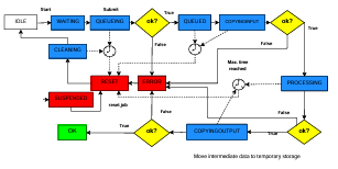
The TaskQ class handles task errors, resets, and time outs in a similar way that other plug-ins do for jobs but also takes additional task states into account. The state diagram for a task is shown in Figure 4.3. Each instance of a TaskQ needs to handle its own garbage collection and set the appropriate states independent of the job being handled by the IceProdDAG instance.
4.1.3 Local Database
A goal of this thesis was to implement most of the new functionality at the plug-in level. The existing database structure assumes a single batch system job ID for each job in a dataset. The same is true for submit directories and log files. Rather than changing the current database structure to accommodate task-level information, a low-impact SQLite database is maintained locally by the TaskQ plug-in in order to keep track of this information. The use of SQLite at the plug-in level had already been established by both PBS and SGE DAGs in order to keep track of the local queue ID information for each task.
4.2 Attribute Matching
A new database table has been added to assign attributes to a particular grid or IceProd instance. These attributes are used in the mapping of DAG tasks to special resources. These attributes are added in the iceprod.cfg configuration file as a set of
name value pairs, which can be numerical or boolean. Examples of such attributes are:
• HasGPU = True
• CPU =True
• Memory = 2000
• HasPhotonicsTables = True
• GPUSPerNode = 4
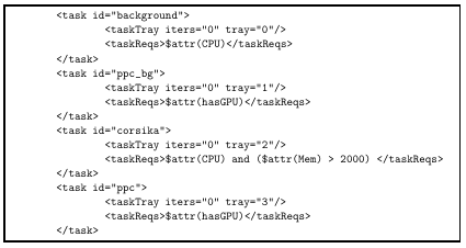
The IceProdDAG does an evaluation of each task requirements and matches them against the attributes advertised by each of the subgrids during each job scheduling interval. The XML schema already included a tag for task requirements that is used to specify Condor requirements or ClassAds directly in the DAGMan plug-in. The expressions for requirements in the IceProd dag are pretty similar to those in Condor and allow for complex boolean expressions involving attribute variables and IceProd expressions as described in Section 2.2.1. A new expression keyword $attr() has been added to the IceProd scripting language for this purpose. The database pivot table (grid statistics) that pairs grids and datasets now includes a new column, task def id, that references a task definition. By default, this column value is set to −1, indicating that this mapping applies to the entire dataset at the job level.
A non-negative value indicates a matching at a specific task level. If an expression evaluates to true when applied to a particular task-grid pair, an entry is created or updated in the grid statistics table. By default, all grids are assumed to have CPUs (unless otherwise specified) and any task without requirements is assumed to require a CPU. Examples of task requirements are shown in Figure 4.4.
4.3 Storing Intermediate Output
Most workflow applications require the passing of data between parent and child nodes in the DAG. One can envision using a direct file transfer protocol between tasks but this is impractical for three main reasons:
1. Firewall rules may prevent such communication between compute nodes.
2. This requires a high level of synchronization to ensure that a child task starts in time to receive the output of it’s parents.
3. With such synchronous scheduling requirements, it is very difficult to recover from failures without having to reschedule the entire DAG.
It is therefore more convenient to define a temporary storage location for holding intermediate out from tasks. A pleasant side effect of this approach is the ability to have a coarse checkpointing from which to resume jobs that fail due to transient errors or that get evicted before they complete. For a local cluster, especially those with a shared file system, this is trivial but on wide-spread grids one should consider bandwidth limitations. In order to optimize performance, an IceProd instance should be configured to use a storage server with a fast network connection. Under most circumstances, this corresponds to a server that has a minimal distance in terms of network hops.
4.3.1 Zones
The concept of a zone ID is introduced in order to optimize performance. Each site is configured with a particular zone ID that loosely relates to the geographical zone where the grid is located. This is an arbitrarily defined numbering scheme and the relative numbers do not reflect distances between zones. For example, University of Wisconsin sites have been assigned a zone ID of 1 and DESY-Zeuthen in Germany has been assigned zone ID 2. A mapping of zone ID to URL is also defined in the configuration file of each instance of IceProd. The distance metric is a measure of
Table 4.1: Example zone definition for an IceProd instance. The IceProd instance in this example is assumed to be located in zone 1.
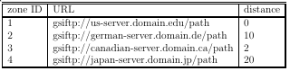
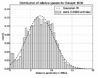
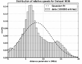
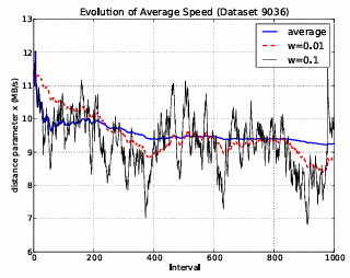
latency with arbitrary units. The distances can be initially assigned arbitrarily at each site in order to minimize network latency. One could in principle just calculate an average network speed for each server. However, in reality, this is a time-dependent value that needs to be optimized periodically. This is accomplished by weighted running average that favors new values over old ones. Figures 4.5 and 4.6 illustrate how the average network speed can vary with time. During a sufficiently short term period, speeds are randomly distributed around mean approximating a Gaussian distribution. Over a longer term, time-dependent factors such as network load can shift mean of distribution so that it no longer resembles a Gaussian. The calculation of the mean value
![]()
(4.1)
can be replaced
![]()
(4.2)
where xi is the distance metric measured a interval i, w < 1 is the weight, and ¯ xi is the weighted running average. The value w = 0.01 was chosen arbitrarily to be sensitive to temporal variation but not too sensitive to high-frequency fluctuations based on Figure 4.7 in an effort to improve performance.
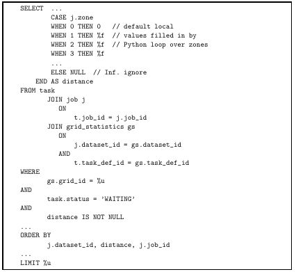
The database has been updated to include a new column “zone” in the job table that is used for determining priorities in scheduling of tasks. Figure 4.8 shows the algorithm for setting priorities in the scheduling of tasks. The distance is periodically calculated based on Equation (4.2) and is used to order the selection of tasks within a dataset from the database. By default, all jobs are initialized to zone 0, which is defined to have a distance of 0.
CHAPTER 5
PERFORMANCE
5.1 Experimental Setup
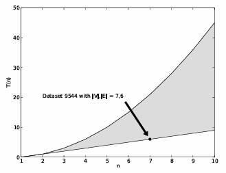
For the purposes of testing the implementation of the IceProdDAG, Dataset 9544 was submitted to IceCube’s production system. This dataset is representative of typical Monte Carlo productions and is represented by the DAG in Figure 5.1. Dataset 9544 consists of 10k jobs that run on CPUs and GPUs and was generated using the 7
separate sites shown on Table 5.1 and distributed throughout in the U.S. and Canada. The test dataset performed at least as well as a batch system driven DAG but allowed for better optimization of resources. The DAG used in Dataset 9544 consists of the following tasks:
1. corsika
generates an energy-weighted primary cosmic-ray shower.
2. background
generates a uniform background cosmic-ray showers with a real is tic spectrum in order to simulate random coincidences in the detector.
3. ppc
propagates photons emitted by corsika. This task requires GPUs.
4. ppc bg
propagates photons emitted by background. This task also requires GPUs.
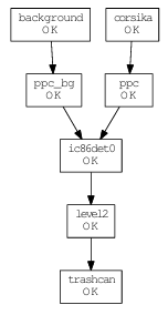
5. ic86det0
combines the output from the two sources and simulates the detector electronics and triggers.
6. level2
applies the same reconstructions and filters uses for real detector data. This task requires the existence of large pre-installed tables of binned multi dimensional probability density functions.
7. trashcan
cleans up temporary files generated by previous tasks.
Sites in Table 5.1 were chosen to test the implementation of the IceProdDAG while minimizing interfere with current Monte Carlo productions. At the same time, it was important that the resources utilized are representative of the those that will be used in a real production environment. The GPU cluster in WestGrid consists of 60 nodes with 3 GPU slots each and is fully dedicated to GPU processing. For this reason, WestGrid is not well suited for standard DAG configurations that rely on the batch system for scheduling tasks and was a driving reason for this thesis. CHTC and NPX3 also include GPUs but are primarily genera-purpose CPU clusters. Each of these sites
Table 5.1: Participating Sites.
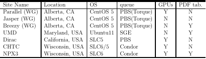
was configured with the appropriate attributes such as HasPhotonics, HasGPU, and CPU to reflect resources listed in Table 5.1. The attribute HasPhotonics indicates that the probability density function (PDF) tables are installed and corresponds to the column labelled “PDF tab.” Appendix E provides more information about each of the sites listed in Table 5.1.
5.2 Performance
5.2.1 Task Queueing
The mechanism for queueing tasks is identical to that of queueing simple serial jobs. As was described in Section 4.2, each grid checks the grid statistics table for dataset,task id pairs mapped to it and queues tasks associated to it.
5.2.2 Task Dependency Checks
The execution time for the dependency checking algorithm described in Section 4.1.1 can be expressed on a per job basis by
T(n,p) = Θ(n ¯ p) (5.1)
where ¯ p is the average number of parents for each task and n is the number of tasks in the DAG. In general, the performance of this algorithm is given by
T(n) = O(n(n−1)/2) (5.2)
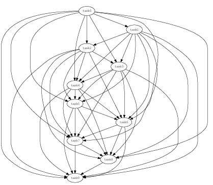
since n(n −1)/2 is the largest number of edges in a DAG size n and each edge needs to be visited. For a DAG of size n, the worst case scenario is given by a maximally connected DAG with ¯ p = (n − 1)/2 such as the one shown in Figure 5.2 where the ith vertex has n − i children. The best case scenario is given by ¯ p = n/(n − 1) ∼ 1 corresponding to a minimally connected DAG such as the one show in Figure 5.3.
which has an execution time given by T(n) = Θ(n) since there are n vertices and n−1 edges as the vertex must have at least one incoming or outgoing edge. The fact that T(n)= Θ(n2/n−1) is due to the fact that every vertex has to be counted once even if it has no parents. The average time for dependency checks is reduced if we use
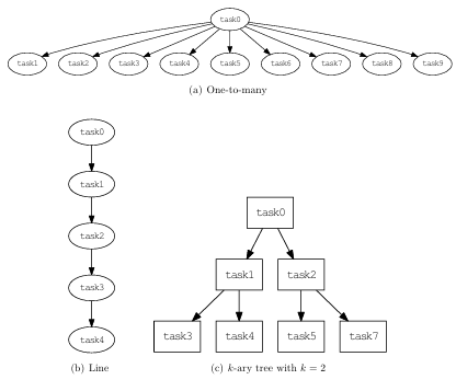
a topologically sorted DAG and exit the loop as soon as we find a task that has not completed. The savings depend on the topology of the particular DAG. For a linear DAG such as the one in Figure 5.3(b), the average number of dependency checks is (n −1)/2 and for for a k-ary tree (Figure 5.3(c)), the average number of checks is
![]()
(5.3)
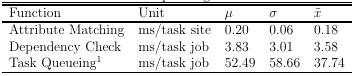
The actual values from the distribution of run times of dependency checks for Dataset 9544 are given in Table 5.2.
5.2.3 Attribute Matching
The algorithm described in Section 4.2 involves periodical checks to see if attributes for sub-grids have changed and subsequent updates to the grid-statistics table. The run time for this algorithm is proportional to the number of tasks in a DAG and the number of sub-grids. The time complexity for matching a dataset to a set of sub-grids is therefore given by
T(nt,ng) = Θ(nt ng) (5.4)
where ng is the number of sub-grids and nt is the number of tasks or vertices in a DAG. This has a similar functional for to that of Equation (5.1). One important difference is that the task dependency check is applied to every queued job where as the attribute matching algorithm described by Equation (5.4) is applied on a per-dataset basis. The actual execution time for each of the algorithms described in Sections 5.2.3, 5.2.1 and 5.2.2 is summarized in Table 5.2.
Table 5.2: Run times for task-queueing functions for Dataset 9544.
5.2.4 Load Balancing
One of the intended benefits of spreading the DAG over multiple sites was to optimize the usage of resources. Given that TaskQ instances are task consumers that pull tasks from the queue (as opposed to being assigned tasks by a master scheduler), each site
1Task queuing only considers database queries and does not include actual batch system calls that can vary significantly from on system to another.
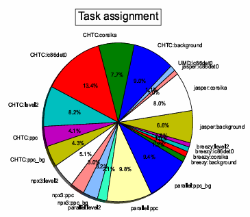
will take what it can consume based on factors such as how many compute slots available or how slow the compute nodes are. This avoids situations in which some clusters is being starved while others are overwhelmed. The pie graph in Figures 5.5,5.6, and 5.7 show the relative number of jobs processed at each of the sites listed in Table 5.1. The larger slices correspond to resources that had the highest throughput during the processing of Dataset 9544.
The performance of DAG jobs is always limited by the slowest component in
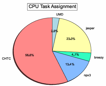
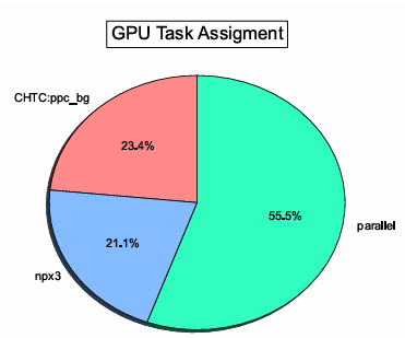
the workflow. The major impetus for this thesis was the concern that simulation production was limited by the small number of GPUs relative to the available CPUs on some clusters and the opposite case for the WestGrid Parallel cluster. This problem can be optimized by pooling resources together as was done with this test run. Table 5.3 shows the run-time numbers for each of the tasks that make up the DAG in Figure 5.1. The ratio of CPU to GPU tasks should roughly be determined by the ratio of
Table 5.3: Run times for tasks in Dataset 9544
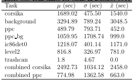
average run times for input CPU tasks to that of GPU tasks plus the ratio of the sum of run times for output CPU tasks to the average runtime of GPU tasks
![]()
(5.5)
which from Table 5.1, we get
Rgpu ≈ 5.84 (5.6)
or using the median instead of the mean,
Rgpu ≈ 6.65 (5.7)
Figure5.8 show the ratio of CPU tasks to GPU tasks during the run of Dataset 9544.Both the median and mean values are high erth an the values given by Equations (5.6)and(5.7), though the value sareske wed by the beginning of the run but seem to approach ¯ Rg puata later point. In reality, the performance of Dataset is affected
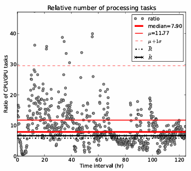
by the variable availability of resources as a function of time.
CHAPTER 6
ARTIFACTS
IceProd is undergoing active development with the aim of improving various aspects of the framework including security, data integrity, scalability, and throughput with the intent to make it generally available for the scientific community in the near future under public licensing.
6.1 Code
Note: The following code and documentation is currently not open to the general public but it will become physically available in the near future.
1. The code for IceProd is currently hosted on IceCube’s Subversion repository:
http://code.icecube.wisc.edu/svn/meta-projects/iceprod
http://code.icecube.wisc.edu/svn/projects/iceprod-core
http://code.icecube.wisc.edu/svn/projects/iceprod-server
http://code.icecube.wisc.edu/svn/projects/iceprod-client
http://code.icecube.wisc.edu/svn/projects/iceprod-modules
6.2 Documentation
1. A wiki containing documentation and a manual is located at
https://wiki.icecube.wisc.edu/index.php/IceProd
2. Epydoc documentation for IceProd Python classes
http://icecube.wisc.edu/~juancarlos/software/iceprod/trunk/
CHAPTER 7
LIMITATIONS OF ICEPROD
7.1 Fault Tolerance
Probably the most important problem with the current design of IceProd is its dependence on a central database. This is a single point of failure that can bring the entire system to a halt if compromised. We have experienced some problems in the past as a result of this. Originally, the IceProd database was hosted on a server that also hosted the calibration database. The load on the calibration database was impacting performance of IceProd. This problem was solved by having a dedicated server.
7.2 Database Scalability
The centralized database also limits the scalability of the system given that adding more and more sites can cause heavy loads on the database server requiring more memory and faster CPUs. This issue and the single point of failure are both being addressed in a second generation design described on Page 61.
7.3 Scope of IceProd
Finally, it should be noted that much of the ease of use of IceProd comes at the price. This is not a tool that will fit every use case. There are many examples that one can come up with where IceProd is not a good fit. However, there are plenty similar applications that can take advantage of IceProd’s design.
CHAPTER 8
CONCLUSIONS
The IceProd framework provides a simple solution to manage and monitor distributed large datasets across multiple sites. It allows for an easy way to integrate multiple clusters and grids with distinct protocols. IceProd makes use of existing technology and protocols for security and data integrity. The details of job submission and management in different grid environments are abstracted through the use of plug-ins. Security and data integrity are concerns in any software architecture that depends heavily on communication through the Internet. IceProd includes features aimed at minimizing security and data corruption risks. The aim of this thesis was to extend the functionality of workflow management directed acyclic graphs (DAGs) so that they are independent of the particular batch system or grid and, more importantly, so they span multiple clusters or grids. The implementation of this new model is currently running at various sites throughout the IceCube collaboration and is playing a key role in optimizing usage of resources. We will soon begin expanding use of IceProdDAGs to include all IceCube grid sites. Support for batch system independent DAGs is achieved by means of two separate plug-ins: one handles the task hierarchical dependencies while the other treats tasks as regular jobs. This solution was chosen so as to minimize changes to the core of IceProd. Only minor changes to the database structure were required.
Asimulation dataset of 10k jobs that run on CPUs and GPUs was generated using 7 separate sites located in the U.S. and Canada. The test dataset was similar in scale to the average IceCube simulation production sets and performed at least as well as a batch system driven DAG but allowed for better optimization of resources. IceProd is undergoing active development with the aim of improving security, data integrity, scalability, and throughput with the intent to make it generally available for the scientific community in the near future. The High Altitude Water Cherenkov Observatory has also recently began using IceProd for off-line data processing.
8.1 Future Work
IceProd has been a success for mass production in IceCube but further work is needed to improve performance. Another collaborator in IceCube is working on a new design for a distributed database that will improve scalability and fault tolerance. Much of the core development for IceProd has been completed at this point in time and is currently being used for Monte Carlo production as well as data processing in the northern hemisphere. Current efforts in the development of IceProd aim to expand its functionality and scope in order to provide the scientific community with a more general-purpose distributed computing tool.
There are also plans to provide support for MapReduce as this may become an important tool for indexing and categorizing events based on reconstruction parameters such as arrival direction, energy, and shape and thus an important tool for data analysis. It is the hope of the author that this framework will be released under a public license in the near future. One prerequisite is to remove any direct dependencies on IceTray software.
REFERENCES
[1] F. Halzen. IceCube A Kilometer-Scale Neutrino Observatory at the South Pole. In IAU XXV General Assembley, Sydney, Australia, 13-26 July 2003, ASP Conference Series, Vol. 13, 2003, volume 13, pages 13–16, July 2003.
[2] Aartsen et al. Search for Galactic PeV gamma rays with the IceCube Neutrino Observatory. Phys. Rev. D, 87:062002, Mar 2013.
[3] J. C. D´ıaz-V´elez. Management and Monitoring of Large Datasets on Distributed Computing Systems for the IceCube Neutrino Observatory. In ISUM 2011 Conference Proceedings., San Lu´ıs Potos´ı, Mar. 2011.
[4] Francis Halzen and Spencer R. Klein. Invited Review Article: Icecube: An Instrument for Neutrino Astronomy. Review of Scientific Instruments, AIP, 81, August 2010.
[5] Tom Weisgarber. personal communication, March 2013.
[6] Andrew Pavlo, Peter Couvares, Rebekah Gietzel, Anatoly Karp, Ian D. Al derman, and Miron Livny. The NMI build and test laboratory: Continuous integration framework for distributed computing software. In In The 20th USENIX Large Installation System Administration Conference (LISA), pages 263–273, 2006.
[7] Dave Winer. XML/RPC Specification. Technical report, Userland Software, 1999.
[8] T R De Young. IceTray: a Software Framework for IceCube. In Computing in High Energy Physics and Nuclear Physics 2004, Interlaken, Switzerland, 27 Sep- 1 Oct 2004, p. 463, page 463, Interlaken, Switzerland, Oct. 2004.
[9] Rick Ellis and the ExpressionEngine Development Team. CodeIgniter User Guide. http://codeigniter.com, online manual.
[10] W Allcock et al. GridFTP: Protocol extensions to FTP for the Grid. http: //www.ggf.org/documents/GWD-R/GFD-R.020.pdf, April 2003.
[11] The Globus Security Team. Globus Toolkit Version 4 Grid Security Infrastruc ture: A Standards Perspective, 2005.
[12] Peter Couvares, Tevik Kosar, Alain Roy, Jeff Weber, and Kent Wenger. Workflow in Condor. In Workflows for e-Science, 2007.
[13] The IceCube Collaboration. Study of South Pole Ice Transparency with Icecube Flashers. In Proceedings of the 32nd International Cosmic Ray Conference, Beijing, China 2011, International Cosmic Ray Conference, Beijing, China, 2011.
[14] D. Chirkin. Photon Propagation Code: http://icecube.wisc.edu/~dima/ work/WISC/ppc. Technical report, IceCube Collaboration, 2010.
[15] J. Cao, S.A. Jarvis, S. Saini, and G.R. Nudd. GridFlow: Workflow Management for Grid Computing, May 2003.
[16] Mark Lutz. Learning Python. O’Reilly & Associates, Inc., Sebastopol, CA, USA, 2 edition, 2003.
[17] Western Canada Research Grid. Parallel QuickStart Guide. http://www. westgrid.ca /support/ quickstart/ parallel, 2013.
[18] NERSC. Dirac GPU Cluster Configuration. http://www.nersc.gov/users/ computational-systems/dirac/node-and-gpu-configuration, 2006.
[19] The CondorHT Team. The Center for Hight Throughput Computing. http: //chtc.cs.wisc.edu, 2011.
[20] Wisconsin Particle and Astrophysics Center. WIPAC Computing. http: //wipac.wisc.edu/science/computing, 2012.
APPENDIX A
PYTHON PACKAGE DEPENDENCIES
An effort has been made to minimize IceProd’s dependency on external Python packages. In most cases, all that is needed is the basic system Python 2.3 (default on RHEL4 or equivalent and above). Only on the server (where daemons run) MySQL-python is also needed. This is not generally included in the system Python. For MySQL, you have two options: request installation of python-MySQL by your system administrator or install the package in a private directory.
The following are the package requirements for IceProd:
1. PyXML 0.8.3 (default on Python 2.3 and above)
2. python-MySQL 1.2.0 (only needed by server)
3. pygtk 2.0.0 (only needed for GUI client, default on Python 2.3 and above)
4. SQLite3 (included in Python ≥ 2.5) or python-sqlite (for Python < 2.5)
In addition, if you want to use SSL encryption (https), you will need pyOpenSSL (server) and Python should be compiled with OpenSSL support (at least for the client). The system Python is typically compiled with OpenSSL support.
APPENDIX B
JOB DEPENDENCIES
For systems without a shared file system (e.g., grid systems), all software dependencies must be shipped to the computing nodes. This file transfer is initiated from the compute node but it can alternatively be done by the submit node. The parameter that controls where data is copied from is lib url. Currently, FTP,HTTP,file (i.e., local system) and GridFTP (if available). If a project needs some external tools or tables that are not part of the meta-project tarball, these must also be sent along with the job. Additional dependencies can be listed in the steering file. This is done through the steering parameter in the section of your xml steering f ile. In the GUI, you can add a dependency in the dependencies tab of the main window. The typical installation of Python on most compute nodes contains all the modules that are needed to run IceProd jobs. However, it is possible to ship Python as a dependency. The JEP can start using a different Python. It will automatically restart itself after downloading and unpacking the Python package dependency. This is done by configuring the pythonhome config parameter to a url rather than a path.
APPENDIX C
WRITING AN I3QUEUE PLUGIN A FOR NEW BATCH
SYSTEM
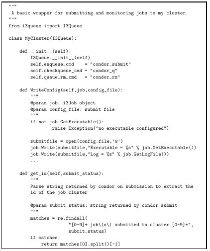
There are already several plug-ins included in IceProd for various batch systems. Developers are encouraged to contribute new plug-ins to the svn repository in order to extend the functionality of IceProd. There are a few methods that need to be implemented but most of the code is simply inherited from I3Queue. The WriteConfig method is the class method that writes the submit script. The most important thing is to define how the submit script for a given cluster is formatted and what are the commands for checking status, queueing, and deleting of jobs. Also, the output from issuing the submit command should get parsed by get id to determine the queue id of this job. Figure C.1 is an excerpt of an I3Queue plug-in implementation.
APPENDIX D
ICEPROD MODULES
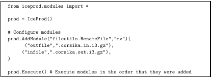
IceProd Modules are Python classes that are executed in a specified sequence. They are configured through similar interface to that of IceTray modules/services.
D.1 Predefined Modules
D.1.1 Data Transfer
The module gsiftp contains the following classes, which are used for transferring files via GridFTP:
1. GlobusURLCopy- for copying individual files
2. GlobusGlobURLCopy- for using wildcard expressions (e.g., *.i3) to copy multiple files
3. GlobusMultiURLCopy- for copying multiple listed files.
APPENDIX E
EXPERIMENTAL SITES USED FOR TESTING
ICEPRODDAG
E.0.2 WestGrid
The WestGrid Parallel cluster consists of multi-core compute nodes. There are 528 12 core standard nodes and 60 special 12-core nodes that have 3 general-purpose GPUs each. The compute nodes are based on the HP Proliant SL390 server architecture, with each node having 2 sockets. Each socket has a 6-core Intel E5649 (Westmere) processor, running at 2.53 GHz. The 12 cores associated with one compute node share 24 GB of RAM. The GPUs are NVIDIA Tesla M2070s, each with about 5.5 GB of memory. WestGrid also provides 1TB of storage accessible through GridFTP, that was used as a temporary intermediate file storage for DAGs [17].
E.0.3 NERSC Dirac GPU Cluster
Dirac is a 50 GPU node cluster. Each node has 8 Intel 5530 Nahalem cores running at 2.4 GHz, and 24 GB RAM divided the following configurations [18]:
• 44 nodes: 1 NVIDIA Tesla C2050 (Fermi) GPU with 3 GB of memory and 448 parallel CUDA processor cores.
• 4 nodes: 1 C1060 NVIDIA Tesla GPU with 4 GB of memory and 240 parallel CUDA processor cores.
• 1node: 4 NVIDIA Tesla C2050 (Fermi) GPU’s, each with 3GB of memory and 448 parallel CUDA processor cores.
• 1 node: 4 C1060 Nvidia Tesla GPU’s, each with 4G B of memory and 240 parallel CUDA processor cores..
E.0.4 Center for High Throughput Computing (CHTC)
CHTCprovides a powerful set of resources summarized on Table E.1 free of charge for University of Wisconsin Researchers and sponsored collaborators. These resources are funded by the National Institute of Health (NIH), the Department of Energy (DOE), the National Science Foundation (NSF), and various grants from the University itself [19].
Table E.1: Computing Resources Available on CHTC
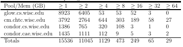
As part of a collaborative arrangement with CHTC, the Wisconsin Particle and Astrophysics Center (WIPAC) added a cluster of GPU nodes on the CHTC network. The cluster, called GZK9000, is housed at the Wisconsin Institutes for Discovery and contains 48 NVIDIA Tesla M2070 GPUs. This contribution was made specifically for IceCube simulations in mind [20].
E.0.5 University of Maryland’s FearTheTurtle Cluster
UMD’s FearTheTurtle consists of a 58 nodes with AMD Opteron processors in the configuration given on Table E.2. The queue is managed by Sun Grid Engine (SGE) and is shared between MC production and IceCube data analysis.
Table E.2: FearTheTurtle Cluster at UMD
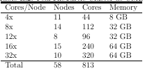
APPENDIX F
ADDITIONAL FIGURES